Tamas Nagy

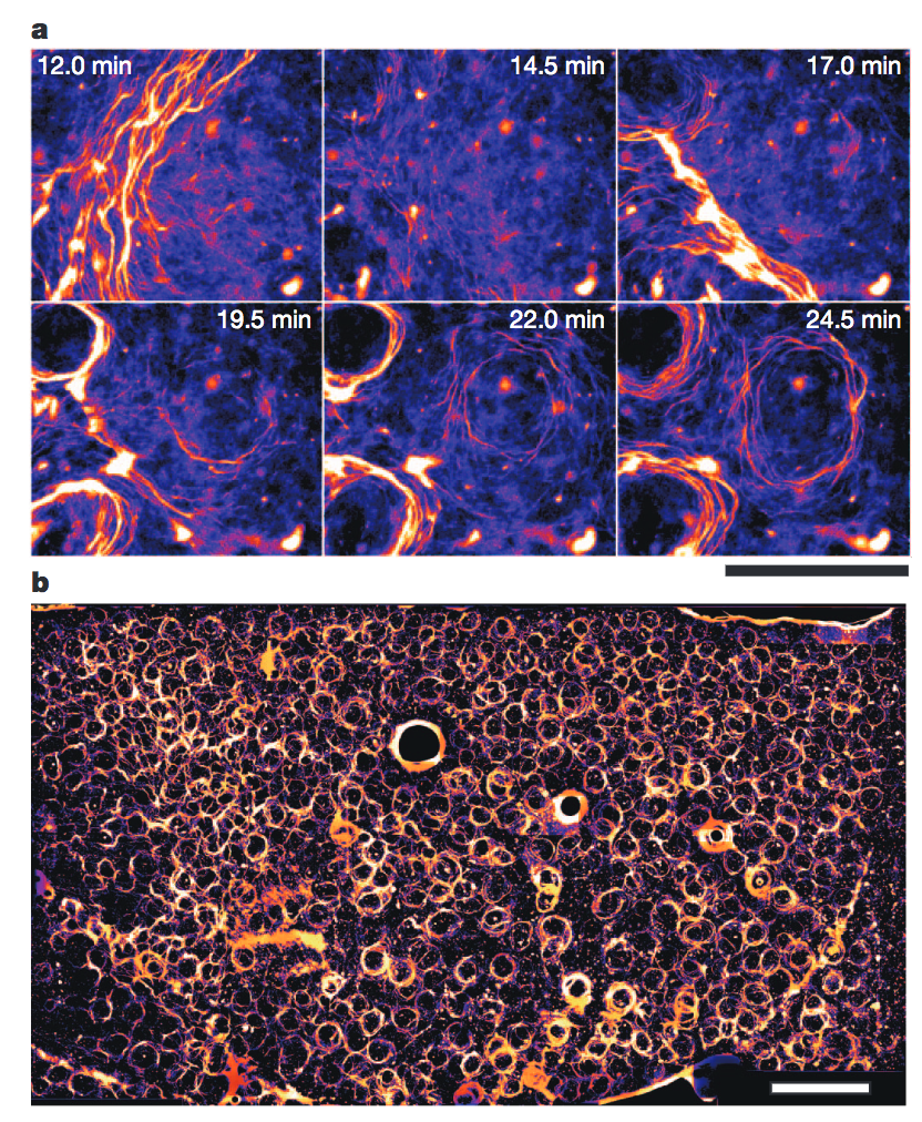
Yesterday was the systems biology module of the iPQB bootcamp here at UCSF. I was in charge of the modeling section and I decided to try to get the students to model the relatively simple active matter system from Sumino et al. (2012) since it was relatively straightforward, very visual, and shows complex emergent properties from simple rules (See Figure 1). Active matter systems are ubiquitous nonequilibrium condensed systems whose “unifying characteristic is that they are composed of self-driven units, active particles, each capable of converting stored or ambient free energy into systematic movement” (Marchetti et al. 2013). An in vitro microtubule and dynein system, like the one we’re investigating here, is much more controlled and reproducible compared to the flocking of birds or fish and thus serves as a nice model system in which to study active matter.

The authors proposed a relatively simple model that could recapitulate this phenomenon. They modeled the behavior of the microtubules as a biased Ornstein–Uhlenbeck process where the microtubules moved at a constant velocity in a direction, \(\theta_i\), that was updated by an angular velocity, \(\omega_i\), at each time step. They added some normal brownian noise to \(\omega_i\) with mean \(\xi_{\mu}\) and standard deviation \(\xi_{\sigma}\). They noticed that the microtubules had a slight clockwise curvature preference and that after relaxation time \(\lambda\), the angular velocity \(\omega_i\) would approach the preferred angular velocity, \(\omega_0\).

Sumino et al. (2012) also noted that microtubules would almost always align or anti-align after collisions (they would sometimes stall or cross). They modeled this by taking the aggregate angle of all neighbors of a microtubule that are within a certain distance from the microtubule. This was then weighted by a parameter \(A\) that controls the relative influence of other microtubules.

Mathematically, this can be expressed in the following non-dimensionalized form:

\[ \begin{align} \frac{d\Omega_i}{dT} &= - \frac{1}{\lambda}\left(\Omega_i - \Omega_0\right) + \textrm{Normal}(\xi_{\mu}, \xi_{\sigma})\\ \frac{d\theta_i}{dT} &= \Omega_i + \frac{A}{N_i(T)} \sum_{j \sim i} \sin\left(2(\theta_j - \theta_i)\right) \\ \frac{d\mathbf{X_i}}{dT} &= \mathbf{e_x}\cos \theta_i + \mathbf{e_y} \sin \theta_i \end{align} \]

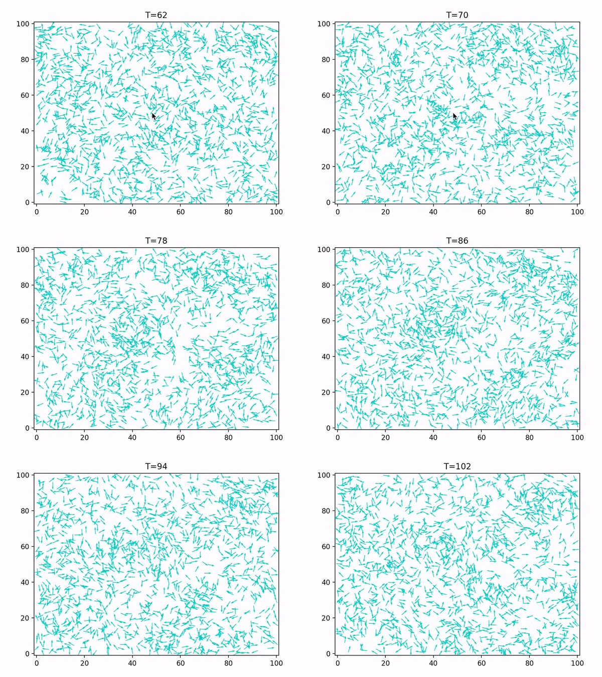
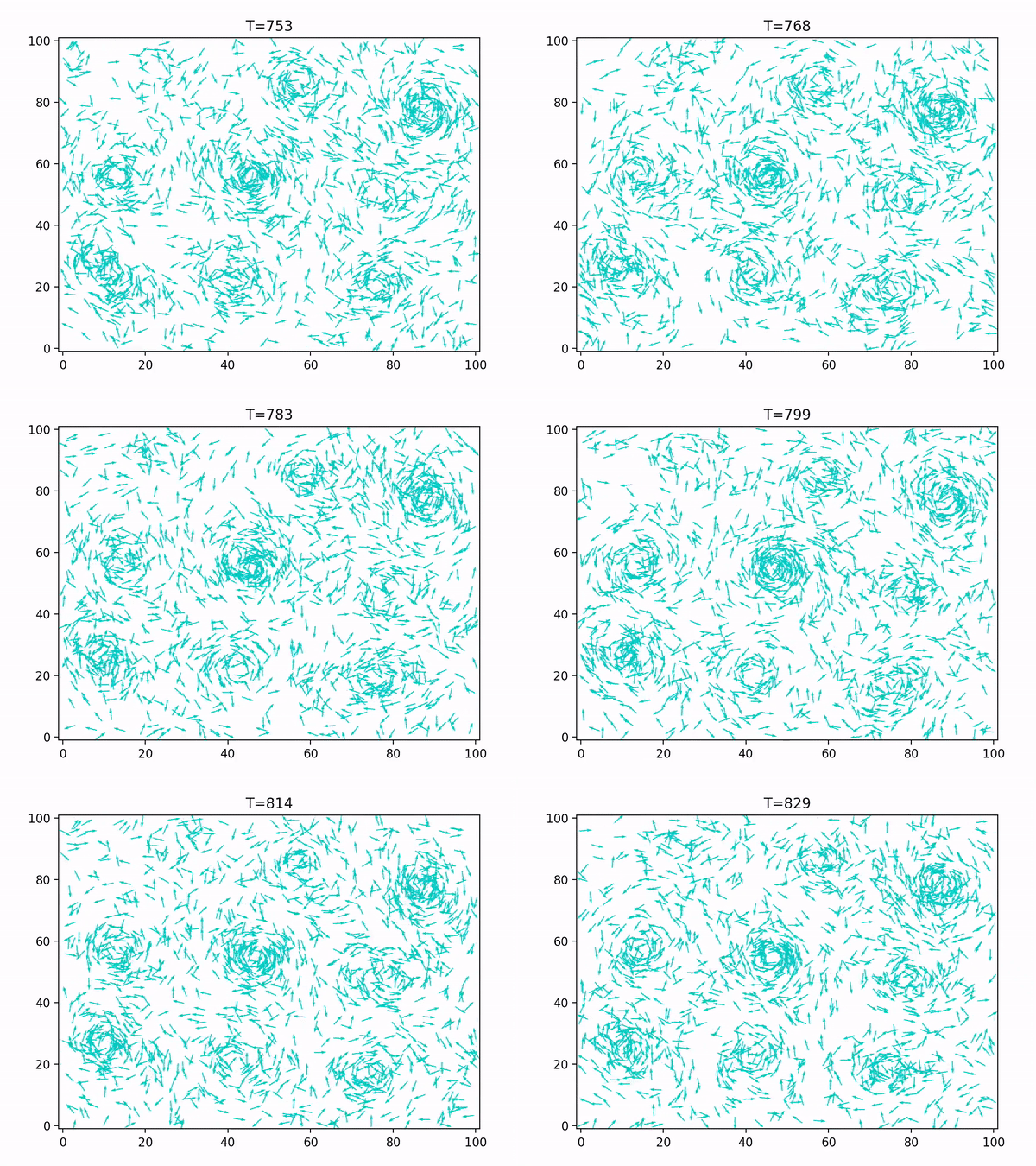
I implemented the code using Python 3, NumPy, SciPy, and Matplotlib and it is available as a Jupyter Notebook in this gist: https://gist.github.com/tlnagy/cba938ffd5c98236e90bfd1dc3d23d11. The students found a quite few parameter combinations that yielded interesting results, most of which were highly unrealistic. I suspect this is due to the much lower “concentration” of microtubules that we used in our simulation to achieve interactivity, \(N=1500\) instead of \(N=2621440\). We were still able to get vortices to form:

References

Marchetti, M. C., J. F. Joanny, S. Ramaswamy, T. B. Liverpool, J. Prost, Madan Rao, and R. Aditi Simha. 2013. “Hydrodynamics of Soft Active Matter.” Rev. Mod. Phys. 85 (3): 1143–89. https://doi.org/10.1103/RevModPhys.85.1143.
Sumino, Yutaka, Ken H Nagai, Yuji Shitaka, Dan Tanaka, Kenichi Yoshikawa, Hugues Chaté, and Kazuhiro Oiwa. 2012. “Large-Scale Vortex Lattice Emerging from Collectively Moving Microtubules.” Nature 483 (7390): 448–52.
Revision history
edited this post on 02 May 2018update links to use https to i can close #7dc3b21c
new post on active modeling45ce9b5